The Big Biddable Guide To Excel Formulas & Shortcuts

Biddable media campaigns create a lot of data. Many times in my career I’ve hit the row limits of excel…

To put that into a number, we’re talking about spreadsheets with more than 1,048,576 rows. Then you have to reach for tools other than excel like GOA Marketing (shameless plug alert).

Excel limits require you to have a lot of data but this is going to happen more and more as digital complexity increases. Data drives business & marketing decisions and helps you invest effectively.

We are all pouring vast sums amounts of money into the coffers of the digital deities of Google & Facebook. (for the record, they aren't technically gods but they are platforms which you can use to reach consumers)

We all want actionable insights. An insight that you can use to optimise your digital marketing campaigns. One that will make a tangible difference to the effectiveness of your advertising.

If you want automated actionable insights then you are in the right place. At GOA, we create dashboards full of useful data. Head over to our information page to check out more….

Anyway, here’s a massive article on excel. Writing this took a very long time and took over my life. There are occasions where you can see I've clearly had too much excel. Yes that's possible. I've thrown in the odd animal and tried to insult various friends who would never read this article.

I’ve categorised this article into these sections, navigate by clicking on the links:

6 useful formulas that that you probably aren’t using This is a selection of useful formulas that I have randomly selected that you (probably) aren’t using. I'm diving in at the deep end to hopefully prove the value of the article to people who have been doing this for years.

Beginners skip these and come back to these formula's at the end.

Introduction to excel formulas

Never forget the mathematical operations

Calculating percentage change

Wildcard Characters in Excel

Error messages in excel

Useful Excel formulas for digital marketing

Matching & looking up data

Validating data

Modifying data

Useful excel features

Pivot tables

Useful keyboard shortcuts for excel

Other useful excel shortcuts

Common excel mistakes

6 useful formulas that that you probably aren’t using

1. LENB - Double Bit Counting LEN

Most people know about LEN, the cell counting formula. Other uses of Baron LEN below but did you know about his sister =LENB ? Chinese, Japanese & Korean ad copy which is double bit needs this slight variation on LEN.

2. How many words are in that cell?

This is more accurately called - how many text or number entries are there in that cell seperated by a cell. It’s not as snappy though is it?

This is useful for ad copy analysis and more. Get this word count formula in your life:

=IF(LEN(A1)=0,0,LEN(A1)-LEN(SUBSTITUTE(A1," ",""))+1)

We’re using four in one here.

LEN counts how many there are including spaces

This LEN SUBSTITUTE combo counts how many characters there are:

=LEN(SUBSTITUTE(A1," ",""))

The +1 that looks like a mistake is actually an important addition. That makes up for the fact that you haven’t included a space at the beginning of your cell... You haven’t have you?!

Finally the IF makes sure that if there is nothing in the cell, then we don’t have a result of 1 (the +1 which counts the first word)

3. Offset. Count all cells to the right and once a blank cell is reached, return the one before

=OFFSET($B2,0,COUNTA($B2:$BZ2)-1,1,1)
    

4. Making plain text into broad match modified keywords

=CONCATENATE("+",SUBSTITUTE(TRIM(A1)," "," +"))
    

There’s another way. Find & replace spaces with ‘ +’ (space+) and then use this formula to add a plus to the beginning:

+”&A1”
    

1. Marking duplicate values in your spreadsheet

=IF(A2=A3,B2+1,1)
    

Cell B2 needs to have a 1 in it to start it off. Then B2 can be copied down

Be sure to check out my other article. The Ultimate Guide On How To Restructure A Paid Search Account

It will help you identify duplicate keywords when creating a restructure.

6. Finding the match type of a keywords from an Google Ads keyword report

This has as many IFs as the trinomial taxonomic name of the Western Lowland Gorilla has Gorillas. Three. See = Gorilla Gorilla Gorilla.

=IF(A1="[","Exact",IF(A1="""","Phrase",IF(A1="+","BMM","Broad")))
    

Introduction to excel formulas

You should be using excel and many of the formulas. If not, you’re wasting a lot of time.

In each formula have the most common usage but don’t be constrained by that. I was always very happy when one of my team found a new use for a formula.

Also combine formulas. This is where the magic happens. I’ll go through most of the useful ones I’ve come across & could remember when writing this article.

Never forget the mathematical operations

Because Excel won’t and it will leave you in a bit of a pickle. Mathematical operations are effectively the order of calculation in a formula

BODMAS (or PEMDAS if you’re from the other side of the pond)

• Brackets (Parenthesis)

• Orders (Exponentials and Roots)

• Division

• Multiplication

• Addition

• Subtraction

Calculating percentage change

Percentage change is the most commonly used one to demonstrate performance changes

Percentage difference is NOT the percentage taken off the total.

Let’s demonstrate this with conversions. Last week we had 10 conversions. This week we have 50. What a great improvement, let’s report that internally. There are two ways of doing the same formula. Here’s the scenario:

Cell C2 has this formula.

=(B2-A2)/A2
    

So that’s this week's conversions, minus last week. This gives you the total difference. You then divide the difference by last weeks.

Another way of getting exactly the same result is this:

=B2/A2-1
    

This week divided by last week gets you the total percentage uplift. Then you minus 1 to subtract the base percentage.

Wildcard Characters in Excel

First off is Asterisk (no Obelix) otherwise known as a *

This can replace characters at the beginning, middle or end of a text string.

TIP- use this in find and replace with a wildcard - Dan* will replace everything after the star. Really useful for modifying URLs etc.

Second is a question mark ?

This can take the place of a single character at the beginning, middle or end of a text string.

Third is tilde ~

This is used to prevent the other two taking action if they are present in your search. So if you wanted to search for * you would search for ~* and ~? If you’re after a question mark.

Error messages in excel

I’m not going to discuss these infuriating messages too long but here are the most common ones you will see. You will get to know and loath them. There are endless articles from Microsoft and other excel gurus on how to fix them. Look it up. Don’t make me LMGTFY.

N/A

Usually because your lookup hasn’t found a matching value.

DIV/0!

Not possible to divide by zero

REF!

The cell you are referring to isn’t valid.

NAME?

You have a text problem. Check quotation marks & that formulas are a-OK

VALUE!

Formula issue.

NUM!

You’ve got a rogue character in your midst. Check to see if you have entered any formatted currency, dates, or special symbols.

Useful Excel formulas for digital marketing

These will all follow a similar pattern. I’ll include the Excel syntax and explain it in my own words with it relating to digital marketing. If you find my version confusing, Excel has a great help section.

Matching & looking up data

IF

Checks whether a condition is met. Returns one value if the formula is matched against (TRUE), and another value if they don’t match (FALSE)

Excel Syntax - IF(logical_test,value_if_true,value_if_false)

• logical_test: slap in your formula or a value here. Anything that has a true and a false. A yin and yang (I always thought Yin had a g at the end, thankfully I checked)

• value_if_true: if the logical_test is matched against and we get a yes or a ‘TRUE’, then Excel will show this result.

• value_if_false: if the test is not matched against so is effectively a NO, not correct or FALSE, then you get this result. If you leave this part of the formula blank then you get this result which is FALSE.

Here’s an example.

Does cell A1 = Badgers?

If yes, then give back the response Huzzah. If not, then Booooooo shall be shown.

=IF(A1="Badgers","Huzzah","Booooooo")
    

Try it out for yourself.

IF doesn’t just have to equal something. It can also be used for greater than, less than and you can also put a AND formula in there to check a range. So to find if the cell has numbers between 50 & 60 do this:

=IF(AND(B5<=60,B5>=50),"Huzzah","Booooooo")
    

VLOOKUP

This is very useful and probably was my most used formula. I was very happy when someone showed me this for the first time. That was until I discovered INDEX MATCH (below) and promptly upgraded. Unfortunately VLOOKUP is like Zoolander in the fact it can’t turn left. And yes, I’m talking about the first film which was great in it’s day, not that second load of rubbish.

VLOOKUP(lookup_value,table_array,col_index_num,range_lookup)

lookup_value: the cell we are looking up. You can include text in the lookup here but you are missing out on the power of this formula if you do that. Reference a cell so you can drag and drop.

table_array: the array we’re looking up. So this is effectively the table you want to pull data back from. This could be a keyword report, a search term output or a weekly report where you reference the Google Ads campaign. Make sure you absolute reference your selection. Why? Absolute reference cells so when you copy / drag / double click this formula, it will still check the correct cells.

col_index_num: is the column number you want the data from. So if it matches, what do you want it to return? The first column in your table_array is number 1.

range_lookup: just put FALSE here. means it’s exact match. As in, I only want this to return me something if the thing I’m looking up to match exactly with my reference cell or whatever my lookup_value is.

Here’s the example I’ll use later with an IFERROR before…. (IFERROR explained just below).

=IFERROR(VLOOKUP(A18,$A$5:$B$10,2,FALSE()),"None Selected")
    

• A18 = the cell we are looking up. The A18 above should really have a $ in front of the A or the 18 depending on where the data is…

• $A$5:$B$10 = The ‘2’ means that we will get the data from column 2. When referencing a larger table, you will spend time counting columns. Now you know why people are pointing at their screen and counting. Particularly towards the end of the day when your eyes are tired.

• FALSE means it’s exact match. As in, the text or number in A18 has to be found exactly for the value to be returned.

IFERROR

Simple one here, but VERY useful. Especially if used with a VLOOKUP (like above) or a INDEX MATCH.

IFERROR(value,value_if_error)

• value: this is a calculation of some description.

• value_if_error: what happens if the value is an error. Can be text or numbers. If text, include in quotation marks (double inverted commas for your US people).

MATCH

If you want to find a cell or some data in a load of cells, then use this formula. This tells you the row in a range of cells where your data matches. No, not like Tinder.

MATCH(lookup_value,lookup_array,match_type)

• lookup_value = reference the cell you want to match. If you reference a cell you can drag this formula around. Or you can put in a value here.

• lookup_array = the array. Effectively the load of cells that you want to search for your lookup_value.

• match_type = 1 finds the largest value & -1 the smallest. 0 finds the first value that is exactly equal to your lookup_value. I almost always put in 0 here.

TIP - always include a match type in MATCH. Otherwise Excel will do what it wants. Well it will include the largest value that is less than or equal to your lookup_value.

INDEX MATCH aka Spicy Combo Meal

Now onto INDEX MATCH. I never use INDEX so I’m going to ignore what it does outside of the polyamorous relationship it has with MATCH. Again, there are loads of examples of INDEX available for your reading pleasure on The Google.

I used to use VLOOKUP until I met INDEX MATCH. I fell for it like my heart was a gangster informer, and the formula was a quiet bit of the thames.

I will follow a different

=INDEX (column to return a value from, MATCH (lookup value, column to lookup against, 0))

We’re going to use INDEX as an array:

And the row_num will be provided by MATCH.

=INDEX($B$5:$B$10,MATCH(A20,$A$5:$A$10,0))
    

Think of it as follows:

INDEX (value you want returned, MATCH (lookup value which should be a cell, column you are matching against, 0 for exact match ))

Then put a IFERROR before and you have a very powerful formula.

=IFERROR(INDEX($B$5:$B$10,MATCH(A17,$A$5:$A$10,0)),"None Selected")
    

INDEX MATCH should be your lookup formula. Not can not only look up to the left or right, it also uses less processing power. VLOOKUP has to check the entire table array and needs to keep on cycling through all your data. INDEX MATCH has a lot less data to check. Think of VLOOKUP as a search and rescue that has very limited information on where you are. INDEX MATCH has a distress signal so knows the rough area. The latter provides considerably quicker results. Maybe not the best analogy but hopefully it helps.

SUMIF

Another really useful formula. You give SUMIF some text, a number or a formula and point it towards a range of cells that you want to add up. Then the formula adds up all the corresponding cells. An example use is to add up all the impressions for exact match keywords.

SUMIF(range,criteria,sum_range)

• range: the total cells that you want evaluated. Let's pretend this is a keyword report that you want to sum up the impressions. Start with the keyword in the far left of your selection and the impressions would be on the far right.

• criteria: this is the criteria for a match to happen.

• sum_range: this is the range of cells that you want to SUM if your criteria is met. Using the example above, it would be impressions.

TIP - SUMIF with wildcard - include a * one one side or either sides to expand your selection. You could use this to search ad copy for a CTA (call to action) and report back the performance data….. Talk to GOA now for example. Subliminal advertising at it’s finest.

SUMIFS

This is an expansion on SUMIF. This is a SUMIF but you can look for multiple criteria… It is useful, try it out. Example use... Find the total impressions for exact match keywords on Google targeting mobile devices.

COUNTIF

This effectively counts the number of cells that meet the criteria you request. E.g. how many exact match keywords are there in this keyword report.

COUNTIF(range,criteria)

• Range: the area you want to count. In the example you could count the match type column. Or the number of square brackets there are. ‘[‘ or ‘]’ not both!

• Criteria: is the lookup value. Can take the form of a number, expression, or text that defines which cells will be counted.

TIP - Like above, COUNTIF can be used with a wildcard.

COUNTIFs

Like SUMIFS, this is the multiple lookup version of COUNTIF. Count the number of match type keywords you have that have a Max CPC higher than £5.

FIND

Use it like a semi VLOOKUP or INDEX MATCH to search for part of a cell. This one is case sensitive, if you don’t want case sensitive then try the next formula…….

SEARCH

Does almost the same as find but doesn’t require the match to be the same case.

So…… Use search if you don’t need the lookup to be case sensitive.

Here’s an example to demonstrate the difference with a cheeky additional ISNUMBER. This will add value to any Medusozoa spreadsheet.

In cell A1 type “Fried Egg Jellyfish” and then put this formula into a spreadsheet:

=IF(ISNUMBER(SEARCH("Fried Egg Jellyfish",A1)),"Great animal name", "This is not a great animal name")
    

You should have the result - Great animal name

Now put “Fried egg Jellyfish” in A1 and copy this formula in:

=IF(ISNUMBER(FIND("Fried Egg Jellyfish",A1)),"Great animal name", "This is not a great animal name")
    

IFNUMBER checks to see if it’s a number in cell A1

I’m going to take a break from longer explanations now. These formulas are useful and are best leveraged with some other ones to do something useful.

TIP - search for “Fried Egg Jellyfish” on Google. It lives up to it's name.

MAX or MIN

Return either the maximum or a minimum value in a range. So these are great with if you combining your MAX or MIN with an IF to look within a range of a range. E.g. to find

NETWORKDAYS

Tells you the number of workdays between two dates. NETWORKDAYS.INT gives you the opportunity to do even more….

These two do the same thing from two different sides. They extra a specified number of characters from the relevant side.

LEFT

Returns X characters from the left.

RIGHT

Returns X characters from the right.

These are really useful for reporting….. Top three orders in a month. Smallest booking in the Congo branch of your hotel chain. Benchmarking your CTR for one country against another. All these and more can be extracted using the below.

LARGE

Returns the Y-th largest value in a data set. If you want to find out the third largest number in a data set, use this formula.

SMALL

You’ve guessed it, this returns the X-th smallest value….

RANK.AVG

Returns the number you’ve specified, as a rank in another list of numbers.

MEDIAN

Use for finding the average AOV when looking at a large range.

TIP - use Median in ad copy testing to find the median when looking at a range of AOVs that two sets of ad copy have compared. eCommerce…..

I don’t really use these that much but they are useful for data validation.

COUNTBLANK

Does what it says… Use this to find out how many blank cells are in that dataset.

COUNTA

The reverse, how many cells have data

TIP - use these two COUNT formulas on your report data validation page... There shouldn’t be any blank or you should have a set number of cells with data……… Validate one page against another. This was meant to go in the paid version of this. I’ve said too much.

Validating data

MATCH

We’ve covered this already but it’s very useful for validating data as well as looking it up.

IF again we’ve covered it but really needed to include it twice as it’s very, very useful. =if(A2=A3,true,false)

IFFY TIP - throw in colour conditioning

Most people know about LEN, the cell character counting formula. Counts all characters in a cell unless you use it with something else.

Other uses of Baron LEN below but did you know about his sister LENB? She's considerably more intelligent. This can count Chinese, Japanese & Korean characters. They are double bit so if you’re validating ad copy for this region, then you need this slight variation on LEN.

Count characters not including spaces:

=LEN(SUBSTITUTE(A2," ",""))
    

Count characters to the left of an underscore:

=LEN(LEFT($B2, SEARCH("_", $B2)-1))
    

If you take the LEN off, it will just return the characters. The LEN counts them.

TIP - modify this with left & right and different characters. Useful for validating tracking URLs

Modifying data

CONCATENATE - I’m sure most of you know this one. It combines multiple cells to make one output. If you want an underscore inbetween your cells, then you need to have this between the cells you want to combine:

,”_”,
    

Swap that underscore out for a space or any other character if required. As always, text needs to be added between quotation marks.

TRIM

You’ve already seen this a few times, use it to get rid of those unwanted spaces either side of your data. Very useful for cleaning your data up.

SUBSTITUTE

Need to replace text in a cell? This is the formula for you. Again, you have seen this but here is the full break down:

SUBSTITUTE(text,old_text,new_text,instance_num)

▪ text: this is the cell that has the text you want to change

▪ old_text: the text you want to replace.

▪ new_text: is the text you want to replace old_text with.

▪ instance_num: which occurrence of old_text do you want replaced? If left blank, then it will do every time. Really useful if the old_text appears multiple times in a cell. You can count the number of times you want it to skip the modifier before it does the ol’switcheroo.

TIP - old_text is case sensitive..... I found this out when reading Excel help writing this article. Or I’m turning senile. At 35, ticking the 35 - 44 demographic box is the closest I’ve come to a midlife crisis thus far.

And after a brief view into my trials & tribulations, onto a bit of rounding….

ROUND

Rounds your number to a specified number of digits

ROUNDUP

Round your number up. Again, you can specify the number of digits.

ROUNDDOWN

Guess what this does? Yes, that’s right, it cooks a perfect poached egg.

Converting dates in Google Analytics

=DATE(LEFT(B8,4),MID(B8,5,2),RIGHT(B8,2))
    

Including text from a dynamic field:

=”New “&B2&”. Shop now!” 
    

More on this below...

Lower, upper & proper

Excel capitilisation forumlas

=EDATE(A1,1)

Add or subtract months with this wonderful little formula. Modify the second number for the action.

TIP - you know you can subtract two dates to find out how many days are in between them? You can also use the aforementioned NETWORKDAYS above.

Useful excel features

Drop down list

A drop down list is great for reporting. To give you an example, I’ve rated a randomly selected group of male names and applied the well known wazzock scale.

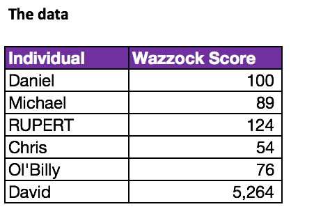
This is the data that we will use

As you can see David is last, but certainly not least.

I’ve created a dropdown bar in the lookup table. This references the other data table to pull back the information.

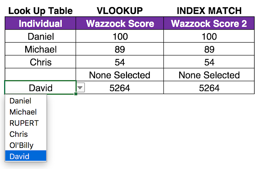
This is the look up table we've created which we can then use either of the below formulas to sum up the data.

The VLOOKUP formula: =IFERROR(VLOOKUP(A18,$A$5:$B$10,2,FALSE()),"None Selected")

This looks the name up and pulls back the corresponding data from the drop down list. If no data is selected like in cell A20, then the IFERROR kicks in and displays None Selected as specified above. I’ll be going through the IFERROR LOOKUP combo in more detail below.

This is the IFERROR INDEX MATCH:

=IFERROR(INDEX($C$5:$C$10,MATCH(B17,$B$5:$B$10,0)),"None Selected")

HINT - use the drop down list as a campaign name identifier to create a dynamic report. Then pull back all the corresponding data in more detail so you can review….

This is all on excel tab - ‘Dropdown List’ in the accompanying excel doc.

Pivot tables

Pivot tables are extremely useful. I somehow managed to go 2 years in paid search without using them, don’t know what I coped. They are not hard once you understand the way they are built. Spend some time learning how to create one because they are ridiculously useful. Your working life will be easier at the end of it. They are great for many reasons, here’s a few:

• You want to present a dataset in a different way - so consolidating data. Maybe you have daily data but you want to show monthly data in one chart and weekly in another.

• You can slice and dice your data to find data patterns or an outlier that needs optimisation. Try pulling a report where you have a campaign fully segmented by hour & day. Then put it into a table that has hours on one side, and days of the week at the the top. Then, with some colour conditioning you can see the times of the day that perform best.

• They take seconds to create. Ok, maybe a minute. It depends on how fast you are (see Excel shortcuts below) but they really are easy when you’ve practiced them.

• They can be updated with very little effort. TIP - save your columns in Google Ads, DoubleClick or Google Analytics. Then output the required CSV anytime you want to pull the data.

A pivot table is made up of rows & columns like any other table but you also get to choose what data fields make up the table. You can segment any bit of data that’s in your report by any other bit of data.

Also be warned. You can very easily create a completely unusable table which tells you nothing.

You can also create a pivot chart which gives you the functionality of a pivot table, but in a chart.

Wooooooaaaaaaaaaaah.

Ok, it’s not that exciting. BUT you harness the power of a pivot chart in action, you will smile and go home earlier than you expected. Or do a better job. Hopefully both.

Other useful pivoty things to know:

• You can filter like you do a normal table.

• Value filter - choose a value (CPA greater than or equal to my target of £10)

• Label filter is how to filter text.

• Report filter does the whole table

You can filter by the following label options:

• Equals

• Does not equal

• Begins with

• Does not begin with

• Ends with

• Does not end with

• Contains

• Does not contain

• Greater than

• Greater than or equal to

• Less than

• Less than or equal to

• Between

And as I’ve just typed that out, I’m going to have to type out the value options you can filter by:

• Equals

• Does not equal

• Greater than

• Greater than or equal to

• Less than

• Less than or equal to

• Between

• Top 10

• Bottom 10

I was going to give some examples on how to use these best but that will have to wait for another day. Definitely apply as much logic as possible but make sure you label what you are filtering by clearly.

Formatting Pivot Tables

You can format your pivot tables just like any other data BUT you must do it this way:

Choose the formatting at the field setting level. Different ways to get there if you’re on a PC or Mac.

I’m on Mac Office 2016. Right click on the column, click on PivotTable Field. Then hit number in the bottom left, and choose your formatting. Then it won’t keep changing and be really annoying!! I have had many frustrating encounters with formatting a pivot table.

There you have it.

DON’T select the cells and click on the formatting at the top. You will be reformatting regularly. No one likes that.

Calculated Fields In A Pivot Table

What do CTR, CPC, Avg Position, Quality Score, Conversion Rate and Revenue per impression have in common? In most pivot tables they need to be created as calculated fields so you can segment your data. For example, you do not want an average CPA or sum of quality score.

Imagine the meeting:

"Yes, that is correct. You have a quality score in the hundreds of thousands for that campaign."

Or, you will have a mild to heavy panic attack when you see your CPA is a few thousand times over the target.

Either way, you don't want this to happen.

Make sure you use calculated fields.

For quality score, average position or any others that aren’t a formula** use the following:

(Impressions x Average position) / Impressions

This will give you the average position however you slice the data.

** I'm referring to CTR being clicks / impressions or conversion rate is conversions / clicks. They are formulas rather than a value.

Grouping data in a pivot table

After creating your pivot table you might want to combine data. An obvious example would be taking daily data and making it into monthly. There are formula ways round this (using MONTH in excel to create another data point) but you can also group. Right click on the made pivot table and select what you're after.

Common issues that people have with a pivot table

• Yes, that’s right. Totals. After a while you will notice that you are inundated with totals. Grand total, sub total. Total this, total that. Too. Many. Totals. You can remove these if you click on your pivot table and navigate to the design section. There you can find subtotals & grand totals. Turn them off if you do not wish to be totalled.

• You add more data, refresh the pivot table. Always do this.

• Sometimes you refresh data but it doesn’t appear in your tables. You need to update your data source. Expand to include the new columns or rows

• If you have no data for a cell, go to ‘Pivot table options’ and update ‘empty cells as:’ to 0 or whatever you want it to be. To find the options, right click on pivot table and there it is. You can also update error cells to be a number but I would address these errors as they could impact your output.

• When you create a pivot table, calculated fields will be named ‘sum of impressions’ or ‘count of match types’. Depending, of course, on what you asked the table to do. The problem is you cannot give two fields the same name. So you need to trick the pivot if you want to give your 'sum of impressions' the name Impressions. The best way to do is to add a space at the beginning or the end of the new name. Then you will have ‘Impressions’ and ‘Impressions ’. The second being the earlier named ‘Sum Of Impressions’

• If you want all the data for a pivot table field then do not fear. Double click on what you want and you get a new table which as all the data that goes into that total.

Colour conditioning

Use colour conditioning to analyse large sways of information. Have simple conditions or use formulas. This is actually called color scales (Grammar police - US English spelling used as it is named so in Excel).

Great for reviewing ad scheduling and more.

Data bars & Icon sets - use these to add a different look to your report.

Tip - use formulas to make these really powerful. I’ll write about this one day.

Useful keyboard shortcuts

There are soooooo many keyboard shortcuts in Excel. You will know many….

The below shortcuts are for a Mac and Excel 2016 so they might be different for the earlier versions. If you use a Mac then make sure you UPGRADE IMMEDIATELY. 2016 actually works. Head here to find the shortcuts for PCs. Usually you can swap out the out the ⌘ below for CTRL.

• Undo - ⌘ +Z

• Redo - ⌘ + Y

• Copy - ⌘ + C

• Paste - ⌘ + V

• Paste Special - ⌘ + CONTROL + V

• Cut - CTRL + X

• Undo - CTRL + Z

• Select All - CTRL + A

• Hold down CTRL to select many items at once

• Navigate to the end of a column - CTRL + arrow

• End of a column or row - CTRL + shift + arrow

• CTRL

• Make the cell absolute reference ($) - F4 or Command + T on Mac

• Hide column(s) - ⌘ + 0

• Hide row(s) - ⌘ + 9

• SUMs the column, row or table you’re messing around with - ⌘ + SHIFT + T

• Turn the number in the cell into a currency - CONTROL + SHIFT + $

• Turn the number into a percentage with no decimal places - CTRL + shift + %

• Turns it into a percentage with two decimal places. (^ is where 6 is) - CTRL + shift + ^ -

• Find - CTRL + F

• Find & Replace - CTRL + H

• Fill down - CTRL + D

• Fill right - CTRL + R

• Add a filter - CTRL + Shift + L or Command + Shift + F

• Insert a hyperlink - CTRL + K

• Enter today’s date - CTRL + semi colon - this is CTRL on PC & Mac.

• Align center - ⌘ + E

• Align left - ⌘ + L

• Select entire column - CONTROL + SPACEBAR

• Select entire row - SHIFT + SPACEBAR

• Select all cells that the formula is using - CONTROL + SHIFT + {

• Move to the next cell in the selection - TAB

Other useful excel shortcuts

Copy formula down with a double click on the bottom right of the cell

Remove duplicates up in the data tab in the top navigation. Find the remove duplicates button.

Common excel mistakes

There are lots potential for mistakes made in pivot tables. There are also lots of mistakes made elsewhere:

• Forgetting to do absolute references

• Not copying a formula all the way down because a filter is applied.

• Formulas can also not be copied if the data in the cell to the left has empty rows.

• Not adding FALSE to VLOOKUP or putting a 0 in a MATCH formula. You won’t get precise matches.

Basic marketing formulas that professionals often get wrong

Calculating the percentage change

I’ve seen so many people, with many years of experience doing this wrong. This is NOT calcuating the percentage difference.

Sale price = Original price x (1 - percent off)

Percent off = 1 - (sales price / original price)

Percentage difference errors! See the beginning of this article.

I have made these mistakes before. Hopefully I haven't done it again!

Calculating media fees and removing fees from your total budget

Ok, you have a media budget of £100,000 for a campaign.

Your agency is taking 15%.

How much is your media budget?

It is not £85,000.

That is removing 15% of £100,000.

To calculate correctly, you need to find the number that if you add 15% to, you will get £100k.

That is very simply done by dividing by 1.15.

Your actual media budget is £86,956.52. Using the other method, you’re slicing just under £2,000 off your campaign. People are not going to be happy.

More guides to excel could follow but for now I am totally done writing about excel for biddable media.

THE END